
How AI Predicts Rainfall 12 Hours in Advance Using Weather Balloon Data — Omdena Case Study
Discover how AI achieved 82% rainfall forecasting accuracy using weather balloon data and XGBoost models in West Africa.
Executive Summary
AI models trained on community-powered weather balloon data achieved 82% accuracy in 12-hour rainfall forecasting across Douala, Cameroon. Existing satellite products operate at resolutions too coarse for localised rainfall events, and traditional weather stations are sparse or absent across large parts of Cameroon, Nigeria, and Ghana. Kanda Weather Group set out to change that by building a low-cost IoT balloon network in which community members launch radiosondes and are compensated for their efforts, producing upper-air atmospheric data that had not existed before.
In a 10-week collaboration with Omdena, a global team of AI engineers turned Kanda’s balloon data into a working 12-hour rainfall forecasting model. Drawing on 1,000+ balloon launches from Douala spanning 2008 to 2020, the team designed three distinct dataset representations, trained seven machine learning architectures, diagnosed and fixed a critical overfitting problem, and applied SHAP explainability to confirm that the model’s learned patterns align with the known atmospheric science of West African rainfall.
XGBoost and CatBoost models achieved the strongest performance on 12-hour rain/no-rain classification, outperforming climatology baselines and delivering results that a portable Docker container now makes available to any partner, on any device, anywhere in West Africa.
When Forecasts Fail: West Africa’s Rainfall Data Gap
For millions of smallholder farmers across Cameroon, Nigeria, and Ghana, rainfall is not a background condition: it is the single most consequential variable in a growing season. A storm arriving six hours earlier than expected can flatten a maize crop. An afternoon downpour on the wrong day can flood an entire district’s harvest. Without a reliable 12-hour forecast, there is no way to act in time.
The reason forecasts fail here is not a modelling problem. It is a data problem. Regional weather prediction depends on a dense network of atmospheric sensors: surface stations, upper-air radiosondes, and satellite instruments capable of resolving local convective events. West Africa has a fraction of what high-income weather systems rely on. The satellites that do cover the region operate at resolutions too coarse to capture the highly localised rainfall patterns that define the Douala climate.
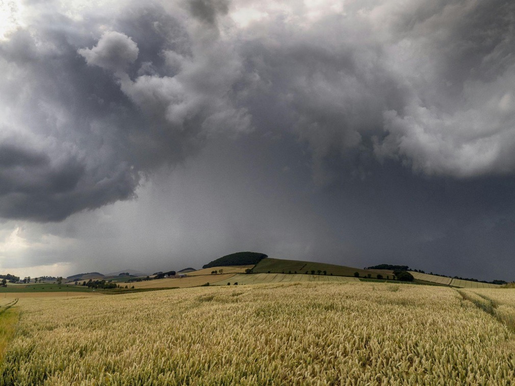
Douala, Cameroon’s largest city, sits at the foot of Mount Cameroon at the edge of the Atlantic, a geography that makes it one of the rainiest cities on Earth, with extreme month-to-month variability. The chart below makes the scale of that variation concrete.
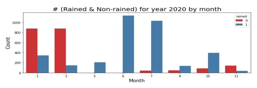
Rain and no-rain distribution by month for Douala, 2020. The contrast between January–February (predominantly no rain) and June–July (overwhelmingly rainy) illustrates the seasonal signal that any useful forecasting model must capture.
Understanding whether it will rain in the next 12 hours requires knowing what is happening right now in the upper atmosphere: the humidity profile at 400 hPa, the thermal lapse rate, and the low-level wind convergence. None of that is available from a standard weather app, and none of it is measured by the sparse surface network that serves most of West Africa.
Kanda Weather Group built a solution from the ground up. Rather than waiting for infrastructure that may take decades to arrive, they designed a low-cost IoT radiosonde: a weather-balloon payload built on open-source hardware, housed in a 3D-printed container, and communicating over a public LoRaWAN network. Each launch costs less than half of a standard radiosonde deployment anywhere else in the world. Community members are paid in convertible digital currency to carry out the launches. The result is a dataset that simply did not exist before Kanda created it.
The Missing Data Layer: How Kanda Built West Africa’s Atmospheric Data Network
A standard weather balloon launch anywhere in Europe or North America uses a factory-sealed radiosonde that costs hundreds of dollars and is operated by trained meteorological staff. Kanda Weather’s approach inverts every one of those assumptions.
The payload is open-source hardware inside a 3D-printed box. The communication runs over LoRaWAN, a low-power public network that requires no dedicated infrastructure. The operator is a resident who receives digital currency for completing the launch. The total cost is less than half that of a conventional radiosonde deployment. The data flows directly into Kanda’s forecasting dashboard, feeding both their existing weather app and the AI model built during this project.
The atmospheric data captured at each launch include pressure, temperature, relative humidity, dew point, and wind direction and speed, sampled at multiple pressure levels as the balloon ascends from the surface to the upper troposphere. The IGRA2 (Integrated Global Radiosonde Archive) format is used for storage and retrieval, providing the data with international scientific credibility and enabling direct comparison with other radiosonde networks worldwide.
The dataset used in this project: 1,000+ balloon launches from Douala, Cameroon, spanning 2008 to 2020, cross-referenced with hourly rainfall observations from the ISD (Integrated Surface Database) to create a binary classification target. Did it rain in the 12 hours following each launch?
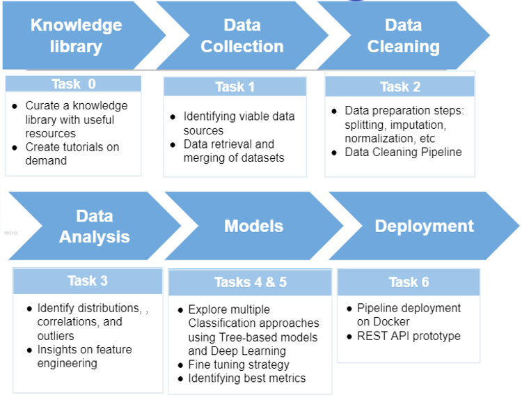
The six-task project pipeline: from knowledge curation and data collection through cleaning, exploratory analysis, model development, and final Docker deployment.
What a Weather Balloon Captures: The Vertical Atmospheric Profile
Each balloon launch captures the vertical profile of the atmosphere above Douala: a column of readings taken at different pressure levels as the balloon climbs from roughly 1,020 hPa near the surface to 400 hPa in the upper troposphere. At every pressure level, the balloon records temperature, relative humidity, and wind speed and direction.
This structure creates a modelling challenge that is more complex than it first appears. A single launch on a single day might generate 10 to 30 rows of data, one per pressure level, but only one rainfall outcome: rain or no rain in the following 12 hours. Any model trained naively on this structure will see multiple copies of the same outcome, interpret each pressure-level reading as an independent event, and overfit dramatically. Diagnosing and fixing this problem became one of the most important technical contributions of the project.
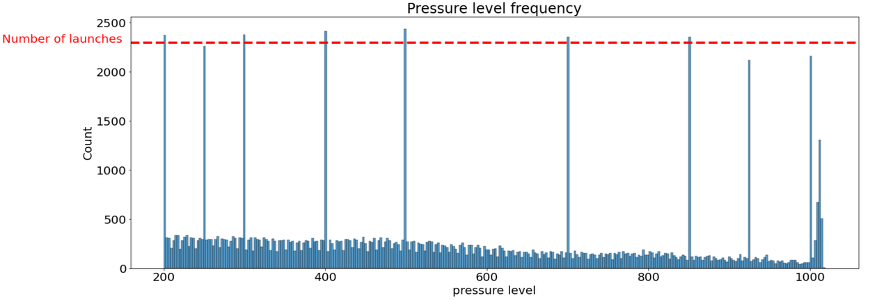
Pressure level frequency across all balloon launches from Douala. The consistent peaks at 200, 400, 500, 700, 850, and 1000 hPa, internationally standardised levels, formed the basis of Dataset 2’s feature engineering.
The team also ran an initial analysis of feature correlations across the raw dataset. Temperature and pressure showed a strong positive correlation (r = 0.97), as expected, since temperature decreases predictably with altitude. Relative humidity correlated at 0.56 with temperature and 0.61 with pressure. These relationships informed the feature engineering strategy that followed.
Three Dataset Representations: Feature Engineering at the Core
Rather than committing to a single data format, the team designed three distinct representations of the same underlying balloon data, each making different trade-offs between sample size, feature richness, and modelling complexity. This multi-representation strategy is one of the most technically sophisticated aspects of the project.
Dataset 1: One Row Per Pressure Level
The raw merged dataset, with each pressure-level reading on its own row. This preserves the maximum number of data points (76,505 rows) but forces any model to predict a rain/no-rain outcome for each pressure reading rather than for each launch. To work around this, the team developed a two-model approach: a first model produces a prediction per pressure level, and a second model aggregates those predictions into a single daily forecast. Results from this approach are presented in the modelling section.
Dataset 2: Launch-Level Aggregation and the Best-Performing Approach
The most important engineering decision of the project. Instead of multiple rows per launch, the team identified the pressure levels recorded most consistently across all launches (200, 400, 500, 700, 850, 925, and 1000 hPa) and pivoted the data so that each launch becomes a single row with separate columns for temperature, humidity, and wind at every level. This reduces the dataset to 1,889 rows but gives each row a clean one-to-one relationship with a rainfall outcome.
A stratified train/test split, stratified by both month and rainfall outcome, ensures that Douala’s seasonal distribution is equally represented in training and test sets. This is the dataset on which the best model achieved its results.
Dataset 3: Derived Climatological Features
A third representation built from high-level climatological derivatives: convective condensation level, mid-level humidity indices, total precipitable water, and seasonality markers. With just 8 features and approximately 1,926 rows, this is the most compact dataset. It produces the richest interpretability signal. SHAP analysis on models trained here confirms that seasonality and convective condensation level dominate the prediction, a finding that aligns directly with the known meteorological drivers of West African convective rainfall.
Diagnosing Overfitting: The Two-Model Solution
One of the most valuable moments in the project was not a model that performed well. It was a model that performed suspiciously well.
Early in the modelling phase, the team trained classifiers on Dataset 1 and observed accuracy scores above 80% with minimal tuning. Given the complexity of rainfall prediction and the dataset’s limited size, these scores were a red flag rather than a milestone. The team investigated and identified the source: because Dataset 1 contains multiple rows per launch date, a standard random train/test shuffle places different pressure-level readings from the same date into both training and test sets. The model effectively memorised the answer during training, only to be tested on a variant of the same question.
Two changes fixed the problem. First, the data was split by year rather than randomly, with years before 2018 used for training and 2018 onward held for testing, ensuring no launch date appears in both sets. Second, a two-model pipeline was developed: one model predicts rain probability at each pressure level, and a second model averages those predictions for each launch date to produce a single daily forecast.
The result: inflated scores came down to honest levels. LightGBM, XGBoost, and CatBoost on Dataset 1 stabilised in the 73–78% range. The Voting Classifier ensemble reached 78%. These numbers could be trusted, and that trust is the foundation on which everything else is built.
This diagnostic process, recognising overfitting, tracing it precisely to the data structure, and engineering a principled fix, is the kind of rigorous ML practice that distinguishes a production-ready pipeline from a research exercise.
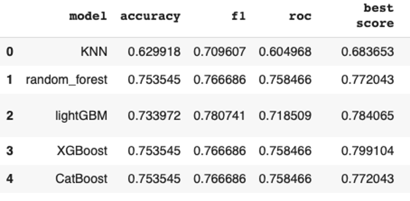
Model performance comparison across five algorithms on Dataset 2 with a stratified train/test split. XGBoost and CatBoost lead with 82% accuracy. LightGBM’s stronger F1 score (0.78) reflects a different precision/recall trade-off on the same dataset.
Model Selection: From Seven Algorithms to One Deployment Choice
With three validated datasets at hand, the modelling team evaluated seven algorithms, ranging from simple baselines to deep learning models.
Algorithms Evaluated
Tree-based models, including Random Forest, XGBoost, LightGBM, and CatBoost, formed the core of the modelling effort. They are well-suited to tabular atmospheric data with mixed numerical features. K-Nearest Neighbours was included as a baseline. The team also ran experiments with convolutional neural networks (CNNs), long short-term memory networks (LSTMs), and gated recurrent units (GRUs).
A significant finding emerged from the deep learning experiments: with fewer than 2,000 training examples in Dataset 2, neural networks lacked sufficient data to learn meaningful representations. Gradient boosting models consistently outperformed them across all three datasets. Neural networks are not always the right tool, and this project demonstrates clearly the conditions under which they are not.
Preprocessing and Splitting Strategy
All models used MinMaxScaler normalisation to bring features onto a common scale, and a log transform to address the class imbalance between rainy days (63%) and dry days (37%). The month variable was one-hot encoded and included as an explicit feature. Early experiments showed it substantially improved accuracy across all models, a signal later confirmed quantitatively by SHAP analysis.
For Dataset 2, stratification by both month and rainfall outcome during train/test splitting was essential. Douala’s climate is bimodal: January and February are predominantly dry, and June through September are overwhelmingly wet. Without stratification, a test set that over-represents dry months would produce misleadingly inflated accuracy scores.
Model Performance
The table below summarises accuracy, F1-score, and ROC-AUC across all evaluated models on Dataset 2 with stratified splitting.
| Model | Accuracy | F1-Score | ROC-AUC | Dataset |
|---|---|---|---|---|
| KNN | 62.3% | 0.71 | 0.60 | Dataset 2 |
| Random Forest | 75.4% | 0.77 | 0.76 | Dataset 2 |
| LightGBM | 80% | 0.78 | 0.77 | Dataset 2 |
| XGBoost ★ | 82% | 0.80 | 0.78 | Dataset 2 (stratified) |
| CatBoost | 82% | 0.79 | 0.79 | Dataset 2 (stratified) |
| Voting Classifier | 78% | — | — | Dataset 1 (ensemble) |
XGBoost on Dataset 2 was selected as the primary model for deployment. It matched CatBoost on accuracy and ROC-AUC, required less hyperparameter tuning, and produced stable results across multiple validation strategies. LightGBM’s stronger F1 score reflects a different precision/recall trade-off rather than overall superiority. For an operational rain warning system, XGBoost’s balance of precision and recall is preferable.
What the Model Learned: SHAP Explainability
Accuracy alone does not make a forecasting model trustworthy. A model that achieves 82% by learning a spurious pattern, whether data entry artefacts, temporal leakage, or coincidental correlations, will not hold up in production. The team used SHAP (Shapley Additive Explanations) to examine what the model learned and to check it against established meteorological science.
The analysis was run on Dataset 3, whose derived climatological features produce the most interpretable SHAP output. The findings are striking in their scientific coherence.
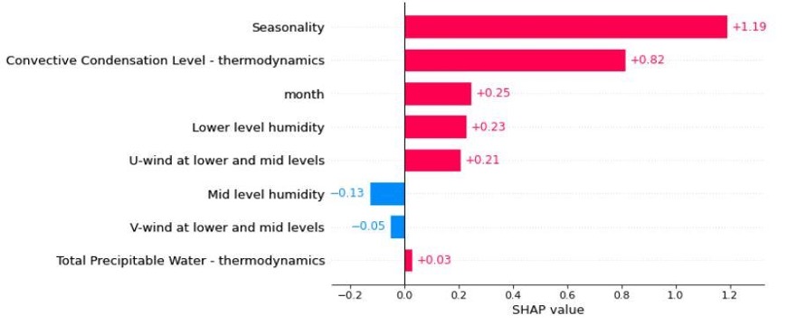
SHAP feature importance for the best model trained on Dataset 3. Seasonality dominates with a mean SHAP value of +1.19, followed by Convective Condensation Level (+0.82) and month (+0.25), all physically meaningful predictors of West African convective rainfall.
Seasonality is the strongest single predictor, with a mean SHAP value of +1.19, far larger than any other feature. This is exactly what meteorological science predicts for Douala: the bimodal rainfall regime is the dominant driver of whether any given day is rainy or dry. The model identified this without being told.
Convective Condensation Level (CCL) follows at +0.82. The CCL is the altitude at which a parcel of surface air, if lifted, would become saturated and begin forming clouds. A low CCL means deep convection, including heavy rain, is energetically accessible. A high CCL means the atmosphere resists convective development. That this thermodynamic parameter ranks second in the SHAP output is precisely what a tropical meteorologist would expect.
Mid-level humidity, lower-level humidity, and U-wind complete the top predictors, each physically interpretable as a contributor to or inhibitor of convective rainfall over coastal West Africa.
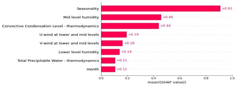
Mean absolute SHAP values across all test instances. Seasonality leads at 0.91, followed by mid-level humidity (0.46) and Convective Condensation Level (0.44), consistent with the bar chart above and reinforcing confidence that the model has captured real atmospheric physics.
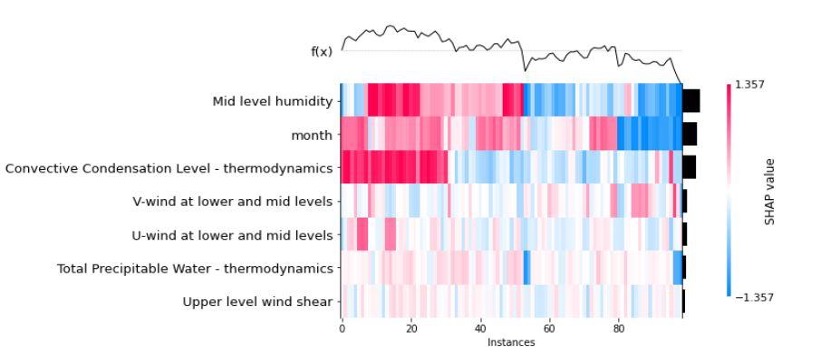
SHAP value heatmap across 100 test instances. Each column is one observation, each row a feature, with red indicating a positive contribution to the rain prediction and blue a negative one. The cluster of high seasonality values on the right corresponds to peak wet-season months, exactly the pattern visible in the raw rainfall distribution.
The consistency of these findings across two independently engineered datasets, Dataset 2 with 38 pressure-level features and Dataset 3 with 8 derived climatological variables, is the strongest signal of model validity. When two different views of the same data agree on which physical processes matter, the model is learning something real.
Results: 82% Accuracy and What It Means
The primary benchmark for this project was climatology: a naive forecast that predicts rain or no rain based purely on historical frequency for the given date. If it rained 6 out of 10 times on 12 July over the previous decade, the climatology forecast assigns 60% rain probability on 12 July of the forecast year. It requires no real-time data and no model, just a lookup table.
Beating climatology is the minimum bar for a useful forecast. The Omdena model cleared that bar on all three datasets, and did so while providing a calibrated probability score and interpretable feature contributions, something a climatology lookup cannot offer.
| Key Results at a Glance |
| XGBoost (Dataset 2, stratified): 82% accuracy · 0.78 ROC-AUC · F1 0.80 |
| CatBoost (Dataset 2, stratified): 82% accuracy · 0.79 ROC-AUC · F1 0.79 |
| Voting Classifier (Dataset 1, ensemble): 78% accuracy across 5 models |
| Deep learning (CNN / LSTM / GRU): did not outperform gradient boosting at this dataset size |
| Original project target: 90% — gap is well-understood and directly addressable with more balloon launches |
The honest assessment: 82% is a strong result given the dataset size. The IGRA2 archive from Douala provides just under 1,900 usable launch events across 12 years, a small sample for a complex classification problem. The path to 90% is straightforward: more balloon launches. Kanda’s network is built to grow, and as the dataset expands, the same pipeline can be retrained to capture finer-grained patterns.
Precision on the rain class is 0.84, meaning that when the model predicts rain, it is correct 84% of the time, a precision level that makes the forecast operationally useful for early warning without generating excessive false alarms.
From Notebook to Product: Docker Deployment and REST API
A model that lives in a Jupyter notebook is not a product. Kanda Weather’s operational requirement was specific: a portable, device-agnostic forecasting tool their team could run without a data scientist present, deployable in Cameroon, usable by a partner in Nigeria, and runnable on a laptop in a field office in Ghana.
The deployment team translated that requirement into a Docker container. Docker packages the entire runtime environment (the trained model, the preprocessing pipeline, and the prediction logic) into a single container that runs identically on any operating system. There is no dependency installation, no Python version conflict, and no environment configuration required. The container starts, receives a new balloon launch as input, and returns a rain/no-rain probability via a REST API call.
Beyond the portable model, the team went beyond the original specification. The codebase is fully modularised and commented, enabling any engineer to extend or retrain it without starting from scratch. New derived features can be added to the input pipeline without breaking the container. External systems can query the model over HTTP, enabling integration with Kanda’s existing weather dashboard. Local storage allows new model versions to be swapped in without rebuilding the container.
The REST API design means that as Kanda’s balloon network expands to new cities, including Lagos, Accra, and Abuja, each new location can immediately query the deployed model with its own radiosonde data. The forecasting infrastructure scales with the data collection network, without new deployment work at each step.
Scaling Across West Africa: What This System Makes Possible
The immediate output is a 12-hour rain/no-rain forecast for Douala. But the architecture built here is not Douala-specific.
The IGRA2 format is a global standard used by hundreds of radiosonde stations worldwide. Any location where Kanda deploys its low-cost balloon network produces data in the same format. The cleaning pipeline, the three dataset representations, the model training, and the Docker deployment can each be re-run for a new city with a new set of historical launches. The model learns the local atmospheric fingerprint and produces locally calibrated forecasts.
For West African agricultural planning, this matters enormously. A 12-hour rainfall forecast issued at 6 am gives a farmer a decision window: whether to harvest today, delay field preparation, or move livestock to higher ground. At the regional level, it provides disaster risk offices with advanced warning of flooding conditions. At the national level, it builds the atmospheric observation record that feeds into longer-range seasonal forecasting models.
The strongest thing this project demonstrates is not the 82% accuracy figure. It is the end-to-end proof of concept: that community-sourced atmospheric data, carefully engineered and rigorously modelled, can produce a forecast that outperforms climatology. For a continent where weather data infrastructure has been treated as an afterthought for decades, that proof of concept is the most important deliverable.
About the Project
This project was carried out over 10 weeks from September to December 2021 as a collaboration between Omdena and Kanda Weather Group. A global team of more than 30 AI engineers and data scientists contributed across six task streams: knowledge curation, data collection, data cleaning, exploratory data analysis, model development, and deployment.
Kanda Weather Group is a West African weather technology company building a low-cost IoT balloon network to bring upper-air atmospheric sensing to communities across the continent. Their platform compensates community members for balloon launches with convertible digital currency, creating a citizen-science model for atmospheric data collection.
Omdena is a global collaborative platform where AI engineers solve high-impact real-world problems in partnership with mission-driven organisations. This project is part of Omdena’s ongoing work on climate resilience and food security across sub-Saharan Africa.


