Applying Machine Learning to Predict Illegal Dumpsites

Just like any other day, we start our morning with a coffee and a snack to go from our favorite bakery. Later on the same day, we check out our mail where we find letters, newspapers, magazines, and possibly a package that just arrived. Finally at night, after a rough week, we decide to go out to have drinks with friends. Sounds like a pretty uneventful day, right?

Except that we produced lots of trash in the form of plastic, glass, paper, ad more.

According to eurostat, it is estimated that an average person in Europe produces more than 1.3 kg of waste per day (in Canada and the USA, it can go up to more than 2 kg). This is equivalent to a person producing 800 kg of trash per year. Now imagine millions of… billions of people doing the same. Every day!

To give you an even clearer perspective: less than 40% of all the waste produced in Europe is recycled — and it is even less across the other continents. Even further, it is estimated that 20% of all generated waste ends up on illegal dumping (s) in Europe, and 50% in Africa.

TrashOut is an environmental project which aims to map and monitor all illegal dumping (s) around the world and to reduce waste generation by helping citizens to recycle more. This is done through a mobile and web application that helps users with locating and monitoring illegal dumping (s), finding the nearest recycling center or bin, joining local green organizations, reading sustainability-related news, and notifying users about updates on their reports.

In this article, we discuss our analysis of illegal dumping (s) across the world, both in local and global scales.

The problem

The problem statement for this project was to “build machine learning models on illegal dumping (s) to see if there are any patterns that can help to understand what causes illegal dumping (s), predict potential dumpsites, and eventually how to avoid them”. We decided to tackle this wordy problem statement by dividing it into three manageable sub-tasks to be worked on throughout the duration of the project:

• Sub-task 1.1: Spatial patterns of existing TrashOut dumpsites
• Sub-task 1.2: Predict potential dumpsites using Machine Learning
• Sub-task 1.3: Understanding patterns of existing dumpsites to prevent future potential illegal dumping (s)

Datasets

• TrashOut: Reports on illegal dumping (s) provided by users through the TrashOut mobile App. For each report, a number of features are recorded, and the most relevant for this analysis were: location (latitude and longitude, city, country, and continent), date, picture, size, and type of waste.
• Open Street Maps (OSM): Geospatial dataset and information on the cities road network, including the type of roads (e.g. motorway, primary, residential, etc)
• Socioeconomic Data and Applications Center (SEDAC): Population density at 1km grid, from which we also calculated the population density gradient to account for population density in the neighboring cells
• FourSquare: Information about nearby venues
• World Bank Indicators, World Bank’s “What a Waste 2.0”, Eurostat, European Commission Directorate-General for Environment: Datasets for socio-economic indicators.
• Non-dumpsites Control Dataset: we generated our own Control Dataset, which was required to train the model on where dumpsites do not occur. For every TrashOut dumpsite location, we selected a pseudo-random location 1 km away and assigned this as a potential non-dumpsite location.

Methods

The first challenge was to identify and extract meaningful information for the spatial analysis from the available datasets. Our assumption was that illegal dumping (s) are more likely to occur in highly populated places, in proximity to main roads and in proximity to venues of interest such as sports venues, museums, restaurants, etc. Based on this assumption, we used the available dataset to extract, for every TrashOut dumpsites as well as for every location of our Non-dumpsite/Control Non-dumpsites, the 17 features described in Table 1:

Sub-task 1.1: Finding existing dumpsites

City-based Analysis of Illegal Dumpsites/ Dumping (s)

We performed an in-depth analysis focused on six shortlisted cities, with the goal to represent different social statuses and geographical locations so all continents were included, and based on the availability of a considerable number of TrashOut dumpsite reports. The cities analyzed were:

• Bratislava, Slovakia (Europe)
• Campbell River, British Columbia (Canada)
• London, UK (Europe)
• Mamuju, Indonesia (Asia)
• Maputo, Mozambique (Africa)
• Torreon, Mexico (Central America)

For the city-based analysis, we accessed the road network information from the OSM dataset by using the Python package OSMnx. This API allows easy interaction with the OSM data without needing to download it, which makes it very accessible in any location around the world. We structured the analysis in a Colab Notebook for consistency and analyzed the following features for each city: distance to three types of roads (motorway, main and residential), distance to the city center, population density, size, and type of waste.

Results for Bratislava

The proportion of TrashOut dumpsites vs. Control Non-dumpsites and their proximity to nearest roads within 1 km is shown in Figure 1, however, the statistical assessment was undertaken within 100 m using the two-proportion Z-test. The three graphs are generated for each road type (motorways, main roads, and residential roads) with the purpose to identify whether dumpsites are more likely to appear in proximity of a specific road type. In Bratislava, around one-fifth of dumpsites were found in proximity to the main road (within 100 m), and these were found more likely to be reported next to the main road (within 100 m) compared to locations of Control Non-dumpsites. However, most dumpsites are not reported on roadsides, and in fact, being further away from a road was found to be a slightly better predictor of where a dumpsite might occur.

Conclusions

Visualizing the distribution of dumpsite reports throughout the city with the spatial analysis undertaken can be informative in preparation to clean up existing dumpsites, as well as for identifying potential new hotspots. The following observations were drawn from this city-level geospatial analysis.

Information about the type and size of dumpsites may be important for local authorities and decision-makers to consider how best to clean up dumpsites. Having a spatial visualization of the locations and characteristics of each dumpsite across each city area, not only helps to inform management efforts to clean up existing dumpsites, but also to try minimizing potential new dumpsites by introducing bins for specific types of waste, or holding events to increase recycling awareness.

Plastic waste is found alongside other types in many dumpsites, which is not surprising. Waste that can be separated occurs simultaneously in reports: domestic and plastic, glass or metal. This might suggest that infrastructure is lacking (i.e. waste collection facilities), or the population is not aware of waste sorting and recycling.

The amount of construction waste in reports for every part of the world suggests that legislation for construction and demolition waste needs to be improved and compliance needs to be checked/assessed in many places. This might suggest that residents find construction waste difficult or costly to dispose of legally, or that construction companies are neglecting their responsibility to clean up.

It is important to stress that we cannot say where dumpsites actually appear, only where they are reported to TrashOut. Dumpsites may be reported with higher frequency in some areas because there are more residents or passersby to report them, regardless of whether there are more dumpsites in those areas.

The use of these tools and analysis will always need to be supported by local knowledge, as well as with the involvement of local municipalities and authorities.

1.2: Predicting potential dumpsites 

Features to train the Machine Learning model

The second subtask focused on creating a Machine Learning model that could predict whether a location is at risk of becoming a dumpsite. Since we have already seen the variables that were considered to be of a strong influence on dumpsites in Table 1, these variables could be used to predict whether a new location could turn into a dumpsite.

When acquiring the venue categories, we set a radius parameter in the Foursquare library until which distance it is supposed to fetch venue categories information. Although we created datasets with radii 500m, 1km, 2km, and 3km, we came upon the conclusion that the 1km radius dataset was the most appropriate one with the best model performance. It was not too near to the location from which the data was being collected therefore not losing any vital information, and at the same time not too far so that irrelevant information needed to be fetched.

The features: Number of Venue Categories, Nearest Venue Categories, and Frequent Venue Categories were only acquired up until 1km from a given location. Moreover, the five nearest venue categories and five most frequent venue categories were acquired for each given location as separate variables. If the Foursquare API failed to acquire not all 5 (or even none in some cases) categories within a 1km radius, then a None string would be placed instead in the empty variables.

A similar approach was taken for the OSM library for the distance to roads features. The value was only collected for roads up till a 1km radius from a location, with the exception of few cases where the API returned a distance slightly beyond 1km.

For the population density feature, our team discussed different approach ideas, and eventually, we decided that, instead of having a singular value for the population density of the given location, the probability of a dumpsite occurring in (or in very close vicinity of) that location is also affected by the surrounding population. Therefore if the location is in the center of a 1×1 square km cell, then the population densities of the eight 1×1 square km cells around the center cell are also considered. This would be a rather good way to see if the dumpsite is in the middle of a highly-populated area, in the outskirts of the city, or in a nowhere land. Using these nine different population densities (with a more weightage on the center cell’s density), a population gradient is calculated for the location which is given to the model as a separate feature in addition to the population density.

These were the 17 features that would be used for the Machine Learning model part of this subtask. But how do we teach the model what a dumpsite is?

Control dataset

We wanted to train a Machine Learning model such that it learns to understand what constitutes a dumpsite in the 17 variables we gathered. We fetched and calculated the features for every one of the approximately 56,000 dumpsites in the TrashOut dataset that we had. However, it is not possible to train a model just by showing it what a dumpsite is. This is because when we show a location that is highly unlikely to become a dumpsite, we want our model to confidently tell us so. An analogous comparison would be to show 56,000 cats to a child and then expect he/she to recognize that a dog is not a cat.

The solution lies in creating a control dataset. In order to teach the Machine Learning model what a dumpsite is, we also need to teach it to understand what a dumpsite is not.

For the sake of simplicity, we can also call the control dataset non-dumpsites. So how do we go about finding non-dumpsites? Any location that is not a dumpsite is in essence a non-dumpsite. However, that will not help the model learn meaningful differences between the two classes: dumpsites and non-dumpsites. Instead, what we can do is find close geographical points to the dumpsites that we already have and use them as the control dataset. Once again, we experimented with multiple distances from the dumpsite to pick these points and found that a distance of 1 km works best. The advantages of choosing these points are:

• The points are close enough to the dumpsites so that there are subtle changes in the features that the model will be able to learn and appropriately map to the two classes.
• The points are not too close so that the model fails to realize key differences between the features of the two classes.
• The points are not so far that there is no correlation between the two classes, therefore, preventing nullification of the purpose of the control dataset.
• When we choose a point near a reported dumpsite, we assume that a location nearby a known dumpsite has active users of the TrashOut app in the area, so if there was no dumpsite report, we assumed there was no dumpsite in that location.

We also took measures to make sure that the non-dumpsite point generated for each dumpsite did not contain another dumpsite, was not in the vicinity of another dumpsite, and was not in a major water body.

The control dataset was made for every dumpsite so that the two classes were balanced for binary classification. Additionally, all the features that were used in the dumpsite dataset were used for the control dataset as well.

Modeling

Our team investigated three different Machine Learning models throughout the project:

1. Random forest classifier — This approach did not work because the model failed to understand the data in a thorough manner and yielded extremely low accuracy. ❌
2. Neural Networks (Dense and Ensemble) — These series of models and its iterations did not work either because the model was tremendously overfitting. It would be unsuitable for real-world purposes. ❌
3. Light Gradient Boosted Model (LGBM) — This model was our final model. It had good accuracy and the minimum generalization error among all three models. ✅

Results

The final accuracy of our model was 80% on the test set. We employed the use of k-fold cross-validation to maximize the accuracy our model could achieve on the test set. We also observed how important the individual features were when it came to classifying a given location to be prone to a dumpsite or not. This analysis was done with the help of SHAPELY and PDP plots as shown in Figure 5 below.

The SHAPELY plot in Figure 5 shows the contribution of each feature towards the prediction. It depicts the importance that each feature has. A high value of importance signifies that the model considers it as a very important factor when determining if a given location is a dumpsite or not. It is indicated that the most important feature of the model for both classes is the distance to the road variable.

The Partial Dependence Plot in Figure 6 helps one understand the effect of a specific variable on the model output. As the value of a feature changes, its effect on the model will also change accordingly. We compute these plots for all the numerical values that we have, to understand its effect on the prediction of the model. The one shown above is the plot analyzing the effect of distance to roads variable. As it can be observed, as the distance from a given location to a major road increases (positive x-axis), the probability that that location is a dumpsite decreases. The soft spike from 1500 m to 2500 m is due to how we manually placed the value of 2500 m in an example when the API could not find a road up till that distance. Regardless, this situation can be manually handled in the deployment implementation.

One of the key achievements of the team was being able to generate a full city heat map of the city of Bratislava (most of our tests were based here) by running the model on more than 700 locations in the city. In the heat map, the actual dumpsites are plotted in blue markers while the roads are marked in black lines (major roads and highways are visibly thicker than minor roads). The spectrum goes from whitish-yellow to dark red with yellow regions resembling a low probability of becoming a dumpsite and the red regions resembling a high probability of becoming a dumpsite. The heat map provides many beneficial usages. For example, municipalities and local authorities can make smaller heat maps for regional neighborhoods to determine which areas are at a high risk of becoming a dumpsite.

Another important variational use of this heat map is to combine it with valuable insights about socio-economic factors, population density, distance to roads, etc. The reason being that even though the model has considerably good accuracy, the wisdom still lies in the intuition of local authorities and municipalities. These officials will be better equipped to analyze key neighborhoods and areas to find the places where there is a major road or highway nearby, has a high population density, and a certain set of venue categories in close proximity. Then, a heat map can be generated for that area and specific regions can be identified which require immediate attention to mitigate the possibility of becoming a dumpsite.

Sub-task 1.3: Preventing future dumpsites

Global analysis of illegal dumpsites/ dumping (s)

In order to analyze illegal dumpsites/ dumping (s) on a global scale, we combined the data from TrashOut with two other datasets:

• What a Waste: For reported global waste production
• World Bank Indicators: For the socio-economic factors that may affect waste

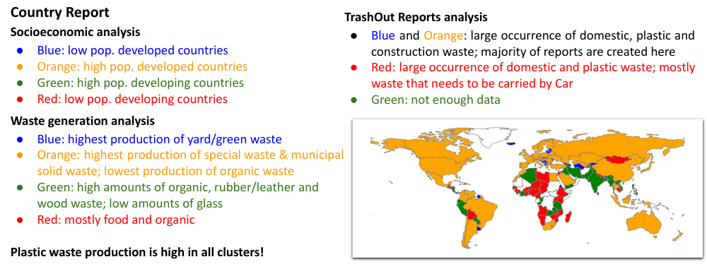
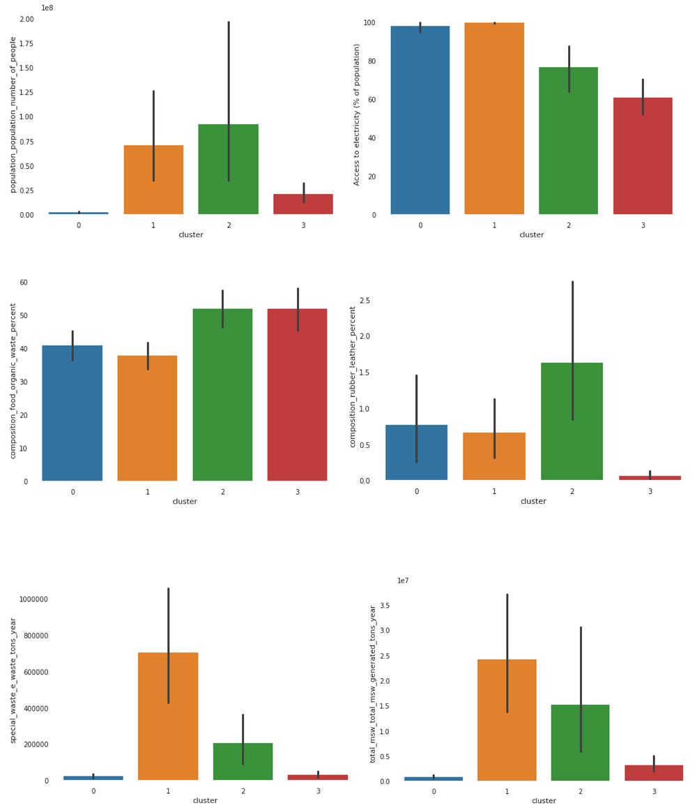
From this setup, it was possible to divide the countries analyzed into four clusters, using unsupervised learning:

Small population developed countries (Blue cluster): countries with a small population and population growth, but high urban populations and access to electricity. These countries also have low urban population growth and GDP. The countries in this cluster present a high production of glass, metal, and paper/cardboard waste, and the highest production of yard/green waste.

High population developed countries (Orange cluster): countries with the highest GDP, and also high access to electricity, urban population, tourism. Low inflation and urban population growth. also produces high amounts of glass and paper/cardboard and is responsible for the highest production of special waste and total municipal solid waste: These countries are also associated with the lowest production of organic waste.

High population developing countries (Green cluster): countries with the highest population and inflation; moderate access to electricity and GDP, and growing urban and total population. They generate high amounts of organic, rubber/leather and wood waste, and low amounts of glass. This can be associated with the high population being less concentrated in cities and also to the level of industrialization of such countries, which may be the ones that most produce factory materials such as leather and rubber.

Small population developing countries/low income (Red cluster): countries with a small population and GDP; lowest electricity access, but highest GDP and population (including urban) growth. Most of the waste produced in these countries is from food and organic sources. These are the countries that also produce the lowest amounts of glass, metal, and rubber/leather waste. Such scenarios can be associated with the low populations and also possible use of waste in a sustainable way, as these countries also present low production of green/yard and wood waste.

Combining this analysis to the illegal dumpsites/ dumping (s) data from TrashOut, our team obtained the following insights:

• Plastic waste is highly produced across all clusters, indicating that this kind of trash needs to have a global awareness strategy.
• Different types of illegal trash are associated with rural and urban areas, making it important on a global scale. Countries with a higher rural population (low income) will produce more illegal organic waste, whereas developed countries present more reports on illegal dumpings/ dumping (s) of plastic, cardboard, yard/green waste, rubber/leather, and special waste.
• Socio-economic factors such as infrastructure, sanitation, inflation, and tourism play a moderate role in the different production of illegal waste worldwide.
• We identify that population is the most important factor in the production of special waste, municipal solid waste, and the total amounts of waste per year. However, most of the special waste produced in developed countries (majority) is reported.

Conclusions

In this project, we have analyzed data on a local and global scale to understand which factors contribute to illegal dumping, as well as predict and finding possible ways to avoid it.

It is important to stress that we cannot say where dumpsites actually appear, only where they are reported to TrashOut. Dumpsites may be reported with higher frequency in some areas because there are more residents or passersby to report them, regardless of the number of dumpsites in those areas.

Nevertheless, visualizing the distribution of dumpsite reports with the spatial analysis undertaken can be informative for identifying potential new hotspots. The following observations can be extracted from our analysis:

On a city level

• The prediction of the ML model and the heatmap can be used as tools for targeted waste management interventions, but will always need to be supported by local knowledge as well as with the involvement of local municipalities and authorities.
• The main road and motorway junctions are locations where illegal disposal of waste is prone to occur. We can witness this in Bratislava and Torreón.
• A lot of reports occur in natural resources areas, e.g. watercourses or natural parks. We can see this in Bratislava, Mamuju, and Campbell River. This may be due to two factors: ease of disposal without being caught; people walking by those areas may be more environmentally aware and wanting to preserve more the places where they go to enjoy nature. Consequently, they create reports more often.
• Waste that can be separated occurs simultaneously in reports: domestic and plastic, glass or metal. This might suggest that infrastructure is lacking (i.e. waste collection facilities), or the population is not aware of waste sorting. This is especially clear in Maputo city.
• The amount of construction waste in reports for every part of the world suggests that legislation for construction and demolition waste needs to be improved and compliance needs to be checked/assessed in many places. This applies to companies and individuals. Construction waste seems to be a problem for many cities.
• TrashOut reports seem to be created in pulses, not on a regular basis. For all the cities examined, there are certain months when the number of reports created exceeds the average by far. Moreover, reports seem to be generally created in specific parts of a city (eg. London).

On a global scale

• Plastic waste production is high across the globe, making it an international problem;
• Among all the socio-economic factors, population plays a strong role in the production of waste in the world (legal and illegal);
• The level of development and socio-economic factors (infrastructure, sanitation, education, among others) play an important role in the kind of waste produced by countries.

In particular:

• Small developed countries present a high production of glass, metal, and paper/cardboard waste, and the highest production of yard/green waste
• High population developed countries: high amounts of glass and paper/cardboard and the highest production of special waste and total municipal solid waste. These countries are also associated with the lowest production of organic waste
• High population developing countries: high amounts of organic, rubber/leather and wood waste, and low amounts of glass;
• Small developing countries/low income: most of the waste produced in these countries is from food and organic sources.

Possible Factors to Avoid Illegal Dumping

• Organization of clean-up events in areas where many dumpsites are already existing can be arranged to clean up the targeted areas in a fun, interactive, and educational way. Collaboration with local authorities should be put in place to improve existing waste infrastructure and build new ones, if necessary.
• Those areas identified as high risk for becoming new potential dumpsites could be targeted with waste infrastructure development/enhancement programs. Additionally, learning events could be organized to raise awareness about dumpsites risks, and how to minimize, or avoid altogether, dumpsites by using properly the waste facility infrastructure existing.
• Examples of learning events consist of learning sessions on how to use waste infrastructure and recycling bins according to local/national authorities, the benefits of a sustainable way of living through the 4R cycle (Refuse, Reduce, Reuse, Recycle), and how to avoid single-use items (or a specific type of waste as can be highlighted by a city-level analysis).

This article is written by Ramansh Sharma, Rosana de Oliveira Gomes, Simone Vaccari, Emma Roscow, and Prejith Premkumar.